Manipulating Large(ish) Datasets with data.table

Author

David Gerard

Published

June 3, 2025

Learning Objectives

Reading large datasets into R.
data.table syntax for manipulating data frames.
A data.table and dplyr tour
Introduction to data.table.
Efficient reshaping using data.tables
Interactive Cheat Sheet

Data Frames and Motivation

Big data: Can’t read data into memory. Need to do distributed computing (like Spark).
Biggish data: Can read data into memory, but it’s very slow to manipulate it.
The data.table package helps you with biggish data.
data.frames are a base R class. We’ve learned about them before.
There are many competitors to data.frames: tibble, DataFrame (from Bioconductor), and data.table.
Julia (another statistical programming language) has its own DataFrames class. Python’s data frame packages are pandas and polars.
data.table is among the fastest in most benchmarks: https://h2oai.github.io/db-benchmark/.
- Python’s polars, and Julia’s DataFrames.jl come close and are faster in some benchmarks.
- dplyr doesn’t come close.
So why did we learn the tidyverse?
- The Posit folks are better at marketing, so dplyr is more widely used.
- For datasets with fewer than, like, one million observations, dplyr works fast enough.

Syntax

Reading in and Printing Data

Load the data.table package and (to compare) the tidyverse into R:
```
library(tidyverse)
library(data.table)
```
We’ll demonstrate most methods with the data from “NYC-flights14” dataset from the data.table package vignettes. I’ve posted it on my own webpage: https://data-science-master.github.io/lectures/data/flights14.csv.
Read in data with fread() (for “file read”). It accepts all delimiters, which you (optionally) specify with the sep argument. The default is to guess the delimiter.
```
flights <- fread("../data/flights14.csv")
```

fread() will return a data.table object.

class(flights)

[1] "data.table" "data.frame"

Use fwrite() to write a data.table object to a file.

Compare to read_csv() in the tidyverse.

flights_tib <- read_csv("../data/flights14.csv")

read_csv() will return a tibble.

class(flights_tib)

[1] "spec_tbl_df" "tbl_df"      "tbl"         "data.frame"

tibbles and data.tables both print better than data.frames.
```
flights
flights_tib
```
You usually use the base function str() (for “structure”) to look at the data.table entries.
```
## data.table way
str(flights)

## Similar tidyverse way
glimpse(flights_tib)
```
You can use as.data.table() to convert a tibble or a data.frame into a data.table. But there is rarely a time when you’d do this, since you use data.table for large datasets that you read in with fread().
```
temp_dt <- as.data.table(flights_tib)
class(temp_dt)
```
```
[1] "data.table" "data.frame"
```

Filtering/Arranging Rows (Observations)

Just like in the tidyverse, we use logicals to filter based on rows. The syntax for this is to place the logicals inside a bracket. Let’s find all flights that left JFK and arrived at LAX.
```
## data.table way
flights[origin == "JFK" & dest == "LAX"]

## equivalent tidyverse way
flights_tib %>%
  filter(origin == "JFK", dest == "LAX")
```

To get a specific row, insert a number into the brackets.

## data.table way
flights[c(1, 3, 207)]

## equivalent tidyverse way
flights_tib %>%
  slice(1, 3, 207)

Reorder rows by using the order() function inside the brackets. Let’s reorder the rows alphabetically by origin, and break ties in reverse alphabetical order by destination.
```
## data.table way
flights[order(origin, -dest)]

## equivalent tidyverse way    
flights_tib %>%
  arrange(origin, desc(dest))
```
Exercise: Use both data.table and the tidyverse to select all flights from EWR and LGA, and arrange the flights in decreasing order of departure delay.

Selecting Columns (Variables)

To select a variable (a column), you also use bracket notation, but you place a comma before you select the columns. This idea is that you are selecting all rows (empty space before comma).
There are lots of ways to select columns that keeps the new object a data.table.

List method: Use the .() function (which is an alias for list()).

## data.table way
flights[, .(origin, dest)]

## Or
flights[, list(origin, dest)]

## equivalent tidyverse way
flights_tib %>%
  select(origin, dest)

Character Vector Method: Use c() with their character names
```
flights[, c("origin", "dest")]
```
Range Method: Use : to select variables within a range of columns.
```
flights[, origin:dest]
```
Prespecify Method: Define variables to keep outside of the data.table, then use with = FALSE. This option makes data.table not think that keep_vec is a varible in the data.table.
```
keep_vec <- c("origin", "dest")
flights[, keep_vec, with = FALSE]
```
To remove a column using the range or character methods, place a ! before the columns to remove
```
flights[, !c("year", "month")]
flights[, !(year:month)]
```
To remove a column using the list method, assign that variable to be NULL using modify by reference (see below). If you run the below code, you’ll need to reload the flights data to get back year and month.
```
flights[, c("year", "month") := .(NULL, NULL)]
```
Exercise: Use data.table to select the year, month, day, and hour columns.

Unlike the tidyverse, you filter rows and select columns in one call rather than using two separate functions.

## data.table way
flights[origin == "JFK" & dest == "LAX", .(year, month, day, hour)]

## equivalent tidyverse way
flights_tib %>%
  filter(origin == "JFK", dest == "LAX") %>%
  select(year, month, day, hour)

Exercise: Use data.table to print out just the departure delays from JFK.

Creating New Variables (Mutate)

The fastest way to create and remove variables in a data.table is by reference, where we modify the data.table, we don’t create a new data.table.

Use := to modify a data.table by reference. You put the variable names (as a character vector) to the left of :=. You put the new variables (as a list) to the right of :=.

## data.table way
flights[, c("gain") := .(dep_delay - arr_delay)]
flights

## equivalent tidyverse way    
flights_tib %>%
  mutate(gain = dep_delay - arr_delay) ->
  flights_tib
flights_tib

Quickly remove a column by setting that variable to NULL.

## data.table way
flights[, c("gain") := .(NULL)]
flights

## equivalent tidyverse way
flights_tib %>%
  select(-gain) ->
  flights_tib
flights_tib

Add multiple variables by separating them with columns.

flights[, c("gain", "dist_km") := .(dep_delay - arr_delay, 1.61 * distance)]
flights

flights[, c("gain", "dist_km") := .(NULL, NULL)]
flights

Exercise: Add a variable called speed that is the average air speed of the plane in miles per hour. Then remove this variable.

Group Summaries

You calculate summaries in the column slot. It’s best to use the list method.

## data.table way
flights[, .(dd = mean(dep_delay))]

## equivalent tidyverse way
flights_tib %>%
  summarize(dd = mean(dep_delay))

## data.table way
flights[, .(dd = mean(dep_delay), ad = mean(arr_delay))]

## equivalent tidyverse way
flights_tib %>%
  summarize(dd = mean(dep_delay), ad = mean(arr_delay))

Count the number of rows with .N.

## data.table way
flights[, .(.N)]

## equivalent tidyverse way
flights_tib %>%
  count()

In data.table, you create grouped summaries by simultaneously grouping and calculating summaries in one line, not separately like in dplyr.

In data.table, you use the by argument to specify the grouping variable. It should also be a list.

## data.table way
flights[, .(dd = mean(dep_delay)) , by = .(origin)]

## equivalent tidyverse way
flights_tib %>%
  group_by(origin) %>%
  summarize(dd = mean(dep_delay))

You can calculate more than one group summary at a time, or group by more than one variable.

## data.table way
flights[, .(dd = mean(dep_delay), .N), by = .(origin, carrier)]

## equivalent tidyverse way
flights_tib %>%
  group_by(origin, carrier) %>%
  summarize(dd = mean(dep_delay), N = n())

`summarise()` has grouped output by 'origin'. You can override using the
`.groups` argument.

Exercise: Use data.table to calculate the median air time for each month.
Exercise: Use data.table to calculate the number of trips from each airport for the carrier code DL.
Exercise: Use data.table to calculate the mean departure delay for each origin in the months of January and February.

Recoding

Suppose you want to change the values of a variable. In the tidyverse, we used recode() to do this.
In data.table, we filter the rows then mutate by reference.

Let’s substitute 24 in hour to 0.

sort(unique(flights$hour))
sort(unique(flights_tib$hour))

## data.table way
flights[hour == 24L, hour := 0L]

## equivalent tidyverse way
flights_tib %>%
  mutate(hour = recode(hour, `24` = 0L)) ->
  flights_tib

sort(unique(flights$hour))
sort(unique(flights_tib$hour))

Exercise: In the origin variable, change "JFK" to "John F. Kennedy", "LGA" to "LaGuardia", and "EWR" to "Newark Liberty".

Gathering

Problem: One variable spread across multiple columns.
Column names are actually values of a variable

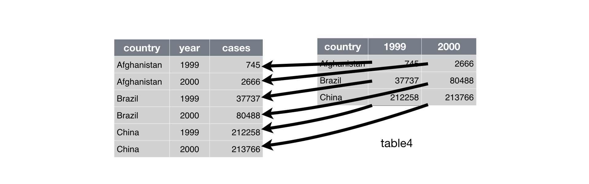
Recall table4a and table4b from the tidyr package

dt4a <- as.data.table(tidyr::table4a)
dt4b <- as.data.table(tidyr::table4b)
dt4a

       country   1999   2000
        <char>  <num>  <num>
1: Afghanistan    745   2666
2:      Brazil  37737  80488
3:       China 212258 213766

dt4b

       country      1999      2000
        <char>     <num>     <num>
1: Afghanistan 1.999e+07 2.060e+07
2:      Brazil 1.720e+08 1.745e+08
3:       China 1.273e+09 1.280e+09

Solution: melt():

## data.table way
melt(dt4a, 
     id.vars       = c("country"),
     measure.vars  = c("1999", "2000"),
     variable.name = "year",
     value.name    = "count")

## Equivalent tidyverse way
tidyr::table4a %>%
  gather(`1999`, `2000`, key = "year", value = "count")

## or
tidyr::table4a %>%
  pivot_longer(cols = c("1999", "2000"), 
               names_to = "year", 
               values_to = "count")

RDS visualization:
Exercise: gather the monkeymem data frame (available at https://data-science-master.github.io/lectures/data/tidy_exercise/monkeymem.csv). The cell values represent identification accuracy of some objects (in percent of 20 trials).

Spreading

Problem: One observation is spread across multiple rows.
One column contains variable names. One column contains values for the different variables.

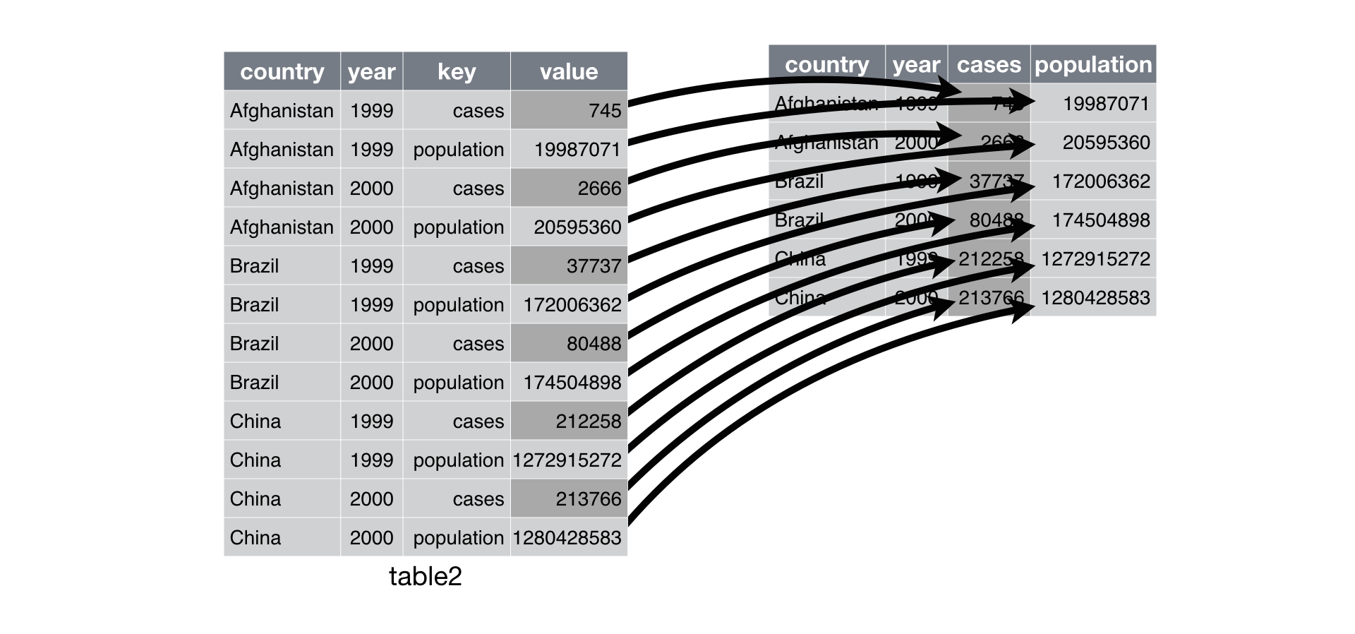
Recall table2 from the tidyr package

dt2 <- as.data.table(tidyr::table2)
dt2

        country  year       type     count
         <char> <num>     <char>     <num>
 1: Afghanistan  1999      cases 7.450e+02
 2: Afghanistan  1999 population 1.999e+07
 3: Afghanistan  2000      cases 2.666e+03
 4: Afghanistan  2000 population 2.060e+07
 5:      Brazil  1999      cases 3.774e+04
 6:      Brazil  1999 population 1.720e+08
 7:      Brazil  2000      cases 8.049e+04
 8:      Brazil  2000 population 1.745e+08
 9:       China  1999      cases 2.123e+05
10:       China  1999 population 1.273e+09
11:       China  2000      cases 2.138e+05
12:       China  2000 population 1.280e+09

Solution: dcast(). In the formula argument, put the “id variables” to the left and the “key” variables to the right. In tidyverse jargon, the value is everything not stated in the formula and the key is everything to the left of the tilde.

## data.table way
dcast(dt2, formula = country + year ~ type, value.var = "count")

## Equivalent tidyverse way
tidyr::table2 %>%
  spread(key = type, value = count)

## or
tidyr::table2 %>%
  pivot_wider(id_cols = c("country", "year"), 
              names_from = "type", 
              values_from = "count")

RDS visualization:
Exercise: Spread the flowers1 data frame (available at https://data-science-master.github.io/lectures/data/tidy_exercise/flowers1.csv).

Separating

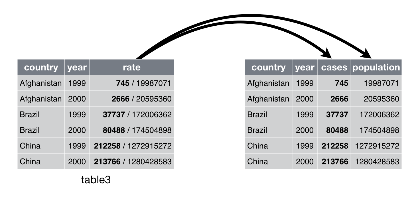
To separate a column into two columns, use the base function tstrsplit().

dt3 <- as.data.table(tidyr::table3)
dt3

       country  year              rate
        <char> <num>            <char>
1: Afghanistan  1999      745/19987071
2: Afghanistan  2000     2666/20595360
3:      Brazil  1999   37737/172006362
4:      Brazil  2000   80488/174504898
5:       China  1999 212258/1272915272
6:       China  2000 213766/1280428583

## data.table way
dt3[, c("cases", "population") := tstrsplit(rate, split = "/")]
dt3[, rate := NULL]
dt3

## equivalent tidyverse way
tidyr::table3 %>%
  separate(rate, into = c("cases", "population"), sep = "/")

RDS visualization:
Exercise: Separate the flowers2 data frame (available at https://data-science-master.github.io/lectures/data/tidy_exercise/flowers2.csv).

Uniting

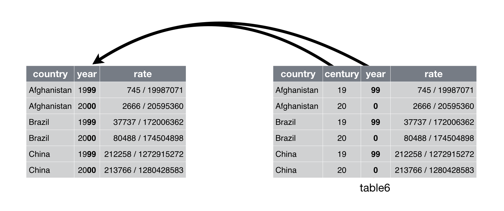
To unite, use paste().

dt5 <- as.data.table(tidyr::table5)
dt5

       country century   year              rate
        <char>  <char> <char>            <char>
1: Afghanistan      19     99      745/19987071
2: Afghanistan      20     00     2666/20595360
3:      Brazil      19     99   37737/172006362
4:      Brazil      20     00   80488/174504898
5:       China      19     99 212258/1272915272
6:       China      20     00 213766/1280428583

## data.table way
dt5[, year := paste(century, year, sep = "")]
dt5[, century := NULL]
dt5

## Equivalent tidyverse way
tidyr::table5 %>%
  unite(century, year, col = "year", sep = "")

RDS visualization:
Exercise: Re-unite the data frame you separated from the flowers2 exercise. Use a comma for the separator.

Chaining

In the tidyverse, we chain commands by using the pipe %>%. In data.table, we chain commands by adding additional brackets after the brackets we used. Data.table makes this very efficient.

Let’s calculate the mean arrival delay for american airlines for each origin/destination pair, then order the results by origin in increasing order, breaking ties by destination in decreasing order.

## data.table way
flights[carrier == "AA", .(ad = mean(arr_delay)), by = .(origin, dest)][order(origin, -dest)]

## Usual indentation for readability:
flights[carrier == "AA", .(ad = mean(arr_delay)), by = .(origin, dest)
        ][order(origin, -dest)]

## Equivalent tidyverse way
flights_tib %>%
  filter(carrier == "AA") %>%
  group_by(origin, dest) %>%
  summarize(ad = mean(arr_delay)) %>%
  arrange(origin, desc(dest))

Joining

We’ll use the following data.tables to introduce joining.

xdf <- data.table(mykey = c("1", "2", "3"),
                  x_val = c("x1", "x2", "x3"))
ydf <- data.table(mykey = c("1", "2", "4"),
                  y_val = c("y1", "y2", "y3"))
xdf

    mykey  x_val
   <char> <char>
1:      1     x1
2:      2     x2
3:      3     x3

ydf

    mykey  y_val
   <char> <char>
1:      1     y1
2:      2     y2
3:      4     y3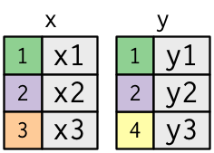

Use the merge() function for all joining in data.table.

Inner Join:

## data.table way
merge(xdf, ydf, by = "mykey")

## equivalent tidyverse way
inner_join(xdf, ydf, by = "mykey")

Outer Joins

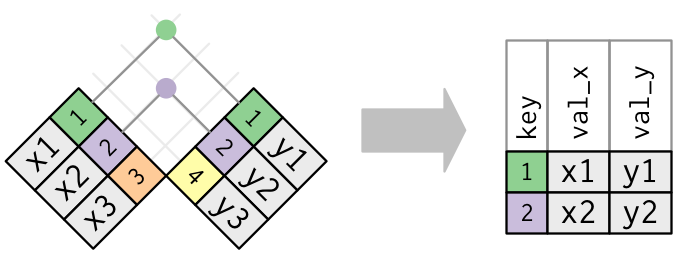
Left Join

## data.table way
merge(xdf, ydf, by = "mykey", all.x = TRUE)

## equivalent tidyverse way
left_join(xdf, ydf, by = "mykey")

Right Join

## data.table way
merge(xdf, ydf, by = "mykey", all.y = TRUE)

## equivalent tidyverse way
right_join(xdf, ydf, by = "mykey")

Outer Join

## data.table way
merge(xdf, ydf, by = "mykey", all.x = TRUE, all.y = TRUE)

## equivalent tidyverse way
full_join(xdf, ydf, by = "mykey")

Binding Rows:

## data.table way
rbind(xdf, ydf, fill = TRUE)

## equivalent tidyverse way
bind_rows(xdf, ydf)

When you have different key names, use the by.x and by.y arguments instead of the by argument.

names(ydf)[1] <- "newkey"
ydf

   newkey  y_val
   <char> <char>
1:      1     y1
2:      2     y2
3:      4     y3

## data.table way
merge(xdf, ydf, by.x = "mykey", by.y = "newkey")

## equivalent tidyverse way
inner_join(xdf, ydf, by = c("mykey" = "newkey"))

Exercise: Recall the nycflights13 dataset

library(nycflights13)
data("flights")
data("airlines")
data("planes")
flights  <- as.data.table(flights)
airlines <- as.data.table(airlines)
planes   <- as.data.table(planes)

Add the full airline names to the flights data.table.

Exercise: Select all flights that use a plane where you have some annotation.

Additional References

There is so much more to data.table. You can do quite complicated and sophisticated data manipulations using data.table that would require a lot more typing in the tidyverse. I am not an expert in much of this functionality. A large number of articles and references are given on the homepage: https://rdatatable.gitlab.io/data.table/.