Learning Objectives

Learn some SQL
Interface SQL with R through the {DBI} and {duckdb} packages.
- Introduction to DBI: https://solutions.posit.co/connections/db/r-packages/dbi/
- DuckDB SQL Introduction: https://duckdb.org/docs/sql/introduction
- DuckDB R API: https://duckdb.org/docs/api/r.html
Write SQL code using the tidyverse and the {dbplyr} package.
- {dbplyr} and SQL: https://dbplyr.tidyverse.org/articles/sql.html
- R for Data Science Database Chapter: https://r4ds.hadley.nz/databases.html

SQL Introduction and Motivation

SQL is pronounced either “ess-kew-ell” or “sequel” (either is fine).
SQL is a programming language which basically allows you to do a lot that dplyr does (filters, selects, joins, etc…). It is the industry standard for interacting with a relational database.
You all are experts in data munging once a dataset has been downloaded.
But, many datasets live in a relational database which is too huge to download onto your computer.
A common task for a data scientist is to download a subset of this huge database so that they can explore it on their computer.
SQL is how you download this subset. You choose which data frames (“tables” in SQL) to download, what subsets of these tables to download (by filtering rows), and whether to join tables together in this process.
We will use R Studio in this lesson. But if you get really into SQL, a popular IDE is DBeaver, with a tutorial from DuckDB here.

DuckDB

There are a lots of database management systems (DBMS) that use SQL to connect to their databases.
In this lecture, we will only consider DuckDB since it has no external dependencies and is pretty easy to install. Just do this in R:

R
```
install.packages("duckdb")
```
The most popular DBMS is probably SQLite. Other popular ones are MySQL and PostgreSQL.
DuckDB is a specific SQL backend. The R package that is used to connect to any SQL backend is {DBI}, and so we will load that one too.

R
```
library(DBI)
library(duckdb)
```

We will compare to the tidyverse:

library(nycflights13)
library(tidyverse)

Let’s download a duck database that I created. Put this in a location you can get to: https://data-science-master.github.io/lectures/data/flights.duckdb
Use duckdb() and DBI::dbConnect() to create a connection to “flights.duckdb”.

R
```
con <- dbConnect(duckdb(dbdir = "../data/flights.duckdb", read_only = TRUE))
```
A basic SQL code chunk looks like this (put SQL code between the chunks):
```
```{sql, connection=con}

```
```

Basic SQL

General

Case does not matter (i.e. select is the same as SELECT is the same as SeLeCt), but it is standard to have all statements be in UPPERCASE (i.e. SELECT).
The statements below must be in the following order: SELECT, FROM, WHERE, GROUP BY, ORDER BY.
New lines and white space don’t matter. But it is common to put those five commands above on new lines.
Character values must be in single quotes.
You can use invalid variable names by putting them in double quotes (same as using backticks in R).
- Some folks always use double quotes because it is not always clear what is an invalid variable name in the database management system. This is what I do below.
Comments in SQL have two hyphens --.
Make sure to put a semicolon ; at the end of a SQL statement. This will allow you to have multiple SQL queries in one chunk.

Showing Tables

The SHOW TABLES command can be used to get a list of all of the tables

SQL
```
SHOW TABLES;
```
5 records

name

airlines

airports

flights

planes

weather

5 records
name
airlines
airports
flights
planes
weather

The DESCRIBE command can be used to show tables and the variables.

SQL

DESCRIBE;

5 records
database	schema	name	column_names	column_types	temporary
flights	main	airlines	carrier, name	VARCHAR, VARCHAR	FALSE
flights	main	airports	faa , name , lat , lon , alt , tz , dst , tzone	VARCHAR, VARCHAR, DOUBLE , DOUBLE , DOUBLE , DOUBLE , VARCHAR, VARCHAR	FALSE
flights	main	flights	year , month , day , dep_time , sched_dep_time, dep_delay , arr_time , sched_arr_time, arr_delay , carrier , flight , tailnum , origin , dest , air_time , distance , hour , minute , time_hour	INTEGER , INTEGER , INTEGER , INTEGER , INTEGER , DOUBLE , INTEGER , INTEGER , DOUBLE , VARCHAR , INTEGER , VARCHAR , VARCHAR , VARCHAR , DOUBLE , DOUBLE , DOUBLE , DOUBLE , TIMESTAMP	FALSE
flights	main	planes	tailnum , year , type , manufacturer, model , engines , seats , speed , engine	VARCHAR, INTEGER, VARCHAR, VARCHAR, VARCHAR, INTEGER, INTEGER, INTEGER, VARCHAR	FALSE
flights	main	weather	origin , year , month , day , hour , temp , dewp , humid , wind_dir , wind_speed, wind_gust , precip , pressure , visib , time_hour	VARCHAR , INTEGER , INTEGER , INTEGER , INTEGER , DOUBLE , DOUBLE , DOUBLE , DOUBLE , DOUBLE , DOUBLE , DOUBLE , DOUBLE , DOUBLE , TIMESTAMP	FALSE

Select Specific Columns

To get the columns from a data frame, use the SELECT command.

The syntax is like this

SQL

SELECT <column1>, <column2>, <column3> 
FROM <mytable>;

Let’s use this to get the tailnum, year, and model variables from the planes table.

SQL

SELECT "tailnum", "year", "model" 
FROM planes;

Displaying records 1 - 10
tailnum	year	model
N10156	2004	EMB-145XR
N102UW	1998	A320-214
N103US	1999	A320-214
N104UW	1999	A320-214
N10575	2002	EMB-145LR
N105UW	1999	A320-214
N107US	1999	A320-214
N108UW	1999	A320-214
N109UW	1999	A320-214
N110UW	1999	A320-214

R equivalent

planes |>
  select(tailnum, year, model)

You select every column by using *:

SQL

SELECT * 
FROM planes;

Displaying records 1 - 10
tailnum	year	type	manufacturer	model	engines	seats	speed	engine
N10156	2004	Fixed wing multi engine	EMBRAER	EMB-145XR	2	55	NA	Turbo-fan
N102UW	1998	Fixed wing multi engine	AIRBUS INDUSTRIE	A320-214	2	182	NA	Turbo-fan
N103US	1999	Fixed wing multi engine	AIRBUS INDUSTRIE	A320-214	2	182	NA	Turbo-fan
N104UW	1999	Fixed wing multi engine	AIRBUS INDUSTRIE	A320-214	2	182	NA	Turbo-fan
N10575	2002	Fixed wing multi engine	EMBRAER	EMB-145LR	2	55	NA	Turbo-fan
N105UW	1999	Fixed wing multi engine	AIRBUS INDUSTRIE	A320-214	2	182	NA	Turbo-fan
N107US	1999	Fixed wing multi engine	AIRBUS INDUSTRIE	A320-214	2	182	NA	Turbo-fan
N108UW	1999	Fixed wing multi engine	AIRBUS INDUSTRIE	A320-214	2	182	NA	Turbo-fan
N109UW	1999	Fixed wing multi engine	AIRBUS INDUSTRIE	A320-214	2	182	NA	Turbo-fan
N110UW	1999	Fixed wing multi engine	AIRBUS INDUSTRIE	A320-214	2	182	NA	Turbo-fan

R equivalent

R
```
planes
```
There is no equivalent for excluding columns (like dplyr::select(-year)). You just select the ones you want.

Filter rows

You use the WHERE command in SQL to filter by rows.

SQL
```
SELECT "flight", "distance", "origin", "dest" 
FROM flights
WHERE "distance" < 50;
```
1 records

flight distance origin dest

1632 17 EWR LGA

1 records
flight	distance	origin	dest
1632	17	EWR	LGA

R equivalent:

flights |>
  select(flight, distance, origin, dest) |>
  filter(distance < 50)

To test for equality, you just use one equals sign.

SQL
```
SELECT "flight", "month" 
FROM flights
WHERE "month" = 12;
```
Displaying records 1 - 10

flight month

745 12

839 12

1895 12

1487 12

2243 12

939 12

3819 12

1441 12

2167 12

605 12

Displaying records 1 - 10
flight	month
745	12
839	12
1895	12
1487	12
2243	12
939	12
3819	12
1441	12
2167	12
605	12

R equivalent

flights |>
  select(flight, month) |>
  filter(month == 12)

For characters you must use single quotes, not double.

SQL
```
SELECT "flight", "origin" 
FROM flights
WHERE "origin" = 'JFK';
```
Displaying records 1 - 10

flight origin

1141 JFK

725 JFK

79 JFK

49 JFK

71 JFK

194 JFK

1806 JFK

1743 JFK

303 JFK

135 JFK

Displaying records 1 - 10
flight	origin
1141	JFK
725	JFK
79	JFK
49	JFK
71	JFK
194	JFK
1806	JFK
1743	JFK
303	JFK
135	JFK

R equivalent

flights |>
  select(flight, origin) |>
  filter(origin == "JFK")

You can select multiple criteria using the AND command

SQL

SELECT "flight", "origin", "dest" 
FROM flights
WHERE "origin" = 'JFK' AND "dest" = 'CMH';

Displaying records 1 - 10
flight	origin	dest
4146	JFK	CMH
3783	JFK	CMH
4146	JFK	CMH
3783	JFK	CMH
4146	JFK	CMH
3783	JFK	CMH
4146	JFK	CMH
3783	JFK	CMH
4146	JFK	CMH
3650	JFK	CMH

R equivalent:

flights |>
  select(flight, origin, dest) |>
  filter(origin == "JFK", dest == "CMH")

You can use the OR logical operator too. Just put parentheses around your desired order of operations.

SQL

SELECT "flight", "origin", "dest" 
FROM flights
WHERE ("origin" = 'JFK' OR "origin" = 'LGA') AND dest = 'CMH';

Displaying records 1 - 10
flight	origin	dest
4146	JFK	CMH
3783	JFK	CMH
4146	JFK	CMH
3783	JFK	CMH
4490	LGA	CMH
4485	LGA	CMH
4426	LGA	CMH
4429	LGA	CMH
4626	LGA	CMH
4555	LGA	CMH

R equivalent

flights |>
  select(flight, origin, dest) |>
  filter(origin == "JFK" | origin == "LGA", dest == "CMH")

Missing data is NULL in SQL (instead of NA). We can remove them by the special command:

SQL
```
SELECT "flight", "dep_delay" 
FROM flights
WHERE "dep_delay" IS NOT NULL;
```
Displaying records 1 - 10

flight dep_delay

1545 2

1714 4

1141 2

725 -1

461 -6

1696 -4

507 -5

5708 -3

79 -3

301 -2

Displaying records 1 - 10
flight	dep_delay
1545	2
1714	4
1141	2
725	-1
461	-6
1696	-4
507	-5
5708	-3
79	-3
301	-2

R equivalent

flights |>
  select(flight, dep_delay) |>
  filter(!is.na(dep_delay))

Just use IS if you want only the missing data observations

SQL
```
SELECT "flight", "dep_delay" 
FROM flights
WHERE "dep_delay" IS NULL;
```
Displaying records 1 - 10

flight dep_delay

4308 NA

791 NA

1925 NA

125 NA

4352 NA

4406 NA

4434 NA

4935 NA

3849 NA

133 NA
When you are building a query, you often want to subset the rows while you are finishing it (you don’t want to return the whole table each time you are trouble shooting a query). Use LIMIT to show only the top subset.

SQL
```
SELECT "flight", "origin", "dest" 
FROM flights
LIMIT 5;
```
5 records

flight origin dest

1545 EWR IAH

1714 LGA IAH

1141 JFK MIA

725 JFK BQN

461 LGA ATL
You can also randomly sample rows via USING SAMPLE:

SQL
```
SELECT "flight", "origin", "dest" 
FROM flights
USING SAMPLE 5 ROWS;
```
5 records

flight origin dest

73 EWR SFO

1421 EWR IAH

1744 LGA IAH

2261 EWR PHX

2054 LGA CLT

Displaying records 1 - 10
flight	dep_delay
4308	NA
791	NA
1925	NA
125	NA
4352	NA
4406	NA
4434	NA
4935	NA
3849	NA
133	NA

5 records
flight	origin	dest
1545	EWR	IAH
1714	LGA	IAH
1141	JFK	MIA
725	JFK	BQN
461	LGA	ATL

5 records
flight	origin	dest
73	EWR	SFO
1421	EWR	IAH
1744	LGA	IAH
2261	EWR	PHX
2054	LGA	CLT

Arranging Rows

Use ORDER BY to rearrange the rows (let’s remove missing values so we can see the ordering)

SQL
```
SELECT "flight", "dep_delay" 
FROM flights
WHERE "dep_delay" IS NOT NULL
ORDER BY "dep_delay";
```
Displaying records 1 - 10

flight dep_delay

97 -43

1715 -33

5713 -32

1435 -30

837 -27

3478 -26

4573 -25

4361 -25

3318 -24

375 -24

Displaying records 1 - 10
flight	dep_delay
97	-43
1715	-33
5713	-32
1435	-30
837	-27
3478	-26
4573	-25
4361	-25
3318	-24
375	-24

R equivalent

flights |>
  select(flight, dep_delay) |>
  filter(!is.na(dep_delay)) |>
  arrange(dep_delay)

Use DESC after the variable to arrange in descending order

SQL
```
SELECT "flight", "dep_delay" 
FROM flights
WHERE "dep_delay" IS NOT NULL
ORDER BY "dep_delay" DESC;
```
Displaying records 1 - 10

flight dep_delay

51 1301

3535 1137

3695 1126

177 1014

3075 1005

2391 960

2119 911

2007 899

2047 898

172 896

Displaying records 1 - 10
flight	dep_delay
51	1301
3535	1137
3695	1126
177	1014
3075	1005
2391	960
2119	911
2007	899
2047	898
172	896

R equivalent

flights |>
  select(flight, dep_delay) |>
  filter(!is.na(dep_delay)) |>
  arrange(desc(dep_delay))

You break ties by adding more variables in the ORDER BY statement

SQL

SELECT "flight", "origin", "dep_delay" 
FROM flights
WHERE "dep_delay" IS NOT NULL
ORDER BY "origin" DESC, "dep_delay";

Displaying records 1 - 10
flight	origin	dep_delay
1715	LGA	-33
5713	LGA	-32
1435	LGA	-30
837	LGA	-27
3478	LGA	-26
4573	LGA	-25
375	LGA	-24
4065	LGA	-24
2223	LGA	-24
5956	LGA	-23

R equivalent

flights |>
  select(flight, origin, dep_delay) |>
  filter(!is.na(dep_delay)) |>
  arrange(desc(origin), dep_delay)

Mutate

In SQL, you mutate variables while you SELECT. You use AS to specify what the new variable is called (choosing a variable name is called “aliasing” in SQL).

SQL
```
SELECT <expression> AS <myvariable> 
FROM <mytable>;
```

Let’s calculate average speed from the flights table. We’ll also keep the flight number, distance, and air time variables.

SQL

SELECT "flight", "distance" / "air_time" AS "speed", "distance", "air_time" 
FROM flights;

Displaying records 1 - 10
flight	speed	distance	air_time
1545	6.167	1400	227
1714	6.238	1416	227
1141	6.806	1089	160
725	8.612	1576	183
461	6.569	762	116
1696	4.793	719	150
507	6.740	1065	158
5708	4.321	229	53
79	6.743	944	140
301	5.312	733	138

R equivalent:

flights |>
  select(flight, distance, air_time) |>
  mutate(speed = distance / air_time)

Various transformation functions also exist:
- LN(): Natural log transformation.
- EXP(): Exponentiation.
- SQRT(): Square root.
- POW(): Power transformation.
  - POW(2.0, x) would be \(2^x\)
  - POW(x, 2.0) would be \(x^2\)
DuckDB is good about implicit coercion. E.g., the following integer division results in a double:
```
SELECT DISTINCT "month", "day", "day" / "month" AS "ratio"
FROM flights
WHERE "month" >= 5
ORDER BY "month", "day";
```
Displaying records 1 - 10

month day ratio

5 1 0.2

5 2 0.4

5 3 0.6

5 4 0.8

5 5 1.0

5 6 1.2

5 7 1.4

5 8 1.6

5 9 1.8

5 10 2.0
But many SQL backends are not so good about implicit coercion.
Use CAST() to convert to a double before operations that should produce doubles.
```
SELECT DISTINCT "month", "day", CAST("day" AS DOUBLE) / CAST("month" AS DOUBLE) AS "ratio"
FROM flights
WHERE "month" >= 5
ORDER BY "month", "day";
```
Displaying records 1 - 10

month day ratio

5 1 0.2

5 2 0.4

5 3 0.6

5 4 0.8

5 5 1.0

5 6 1.2

5 7 1.4

5 8 1.6

5 9 1.8

5 10 2.0
Mutating over partition can be done with OVER (PARTITION BY <variable>). E.g., here is how you find the flight numbers for the longest flights (in terms of air time) from each airport
```
SELECT "flight", "origin", "air_time"
FROM
(
  SELECT "flight", "origin", "air_time", MAX("air_time") OVER (PARTITION BY "origin") AS "amax"
  FROM flights
)
WHERE "air_time" = "amax"
```
3 records

flight origin air_time

51 JFK 691

15 EWR 695

745 LGA 331
In the above, I chained two SQL queries. Your FROM statement can be the output of another SQL query surrounded by parentheses.

Displaying records 1 - 10
month	day	ratio
5	1	0.2
5	2	0.4
5	3	0.6
5	4	0.8
5	5	1.0
5	6	1.2
5	7	1.4
5	8	1.6
5	9	1.8
5	10	2.0

Displaying records 1 - 10
month	day	ratio
5	1	0.2
5	2	0.4
5	3	0.6
5	4	0.8
5	5	1.0
5	6	1.2
5	7	1.4
5	8	1.6
5	9	1.8
5	10	2.0

3 records
flight	origin	air_time
51	JFK	691
15	EWR	695
745	LGA	331

Group Summaries

SQL has a few summary functions (SQL calls these “Aggregates”)
- COUNT(): Count the number of rows.
- AVG(): Calculate average.
- MEDIAN(): Median (not standard across all DBMS’s).
- SUM(): Summation.
- MIN(): Minimum.
- MAX(): Maximum.
- STDDEV(): Standard deviation.
- VARIANCE(): Variance
By default, all missing data are ignored (like setting na.rm = TRUE).
These are calculated in a SELECT command
Let’s calculate the average departue delay

SQL
```
SELECT AVG("dep_delay") AS "dep_delay" 
FROM flights;
```
1 records

dep_delay

12.64

1 records
dep_delay
12.64

R equivalent:

flights |>
  summarize(dep_delay = mean(dep_delay, na.rm = TRUE))

Use the GROUP BY command to calculate group summaries.

SQL
```
SELECT "origin", AVG("dep_delay")
FROM flights
GROUP BY "origin";
```
3 records

origin avg(dep_delay)

JFK 12.11

LGA 10.35

EWR 15.11

3 records
origin	avg(dep_delay)
JFK	12.11
LGA	10.35
EWR	15.11

R equivalent

flights |>
  select(origin, dep_delay) |>
  group_by(origin) |>
  summarize(dep_delay = mean(dep_delay, na.rm = TRUE))

You can get distinct rows by using the prefix DISTINCT in a SELECT statement. E.g. the following will pick up all unique origins
```
SELECT DISTINCT "origin" 
FROM flights;
```
3 records

origin

LGA

EWR

JFK

3 records
origin
LGA
EWR
JFK

Creating Grouped Summaries without Grouping the Results

This section is based on Richard Ressler’s notes.
There may be times when you want to add a grouped summary to the data without collapsing the data into the groups.
As an example, you want to calculate the total departure delay time for each destination so you can use it to then calculate the percentage of that departure delay time for each airline flying to that destination.
You could do that with a summarized dataframe and then a join.
in R, this can be done by using mutate() instead of summarize() to add a new column to the data frame while preserving all of the rows.
In SQL, you have to indicate you want to use the aggregate function as a Window Function to combine grouped aggregated and non-aggregated data into a single result-set table.
When operating as a window function, the table is partitioned into sets of records based on a Field.
Then, the aggregate function is applied to the set of records in each partition and a new field is added to the record with the aggregated value for that partition.
To use an aggregate function as a window function, use the OVER clause with a (PARTITION BY myfield) modifier.

Here is how you find the flight numbers for the longest flights (in terms of air time) from each airport.

SQL

SELECT
    "flight",
    "origin",
    "air_time",
    MAX("air_time") 
    OVER (PARTITION BY "origin") AS "amax"
FROM
    flights
LIMIT 10 OFFSET 120827;

Displaying records 1 - 10
flight	origin	air_time	amax
1100	EWR	324	695
449	EWR	82	695
4382	EWR	87	695
4691	EWR	114	695
1037	EWR	330	695
1266	EWR	301	695
1199	EWR	38	695
3709	EWR	114	695
4407	EWR	164	695
580	EWR	192	695

Note the amax field is new and the values are all the same for the records for each origin.
See SQL Window Functions or SQL PARTITION BY Clause overview for other examples.
This approach can be useful as a sub-query (or inner nested query) inside the outer query FROM clause.

Here is how you find the flight numbers and destination for the longest flights (in terms of air time) from each airport after using the sub-query to find the longest air time from each origin.

SQL

SELECT
    "flight",
    "origin",
    "dest",
    "air_time"
FROM
    (
    SELECT
        "flight",
        "origin",
        "dest",
        "air_time",
        MAX("air_time") OVER (PARTITION BY "origin") AS "amax"
    FROM
        flights
)
WHERE
    "air_time" = "amax"

3 records
flight	origin	dest	air_time
51	JFK	HNL	691
15	EWR	HNL	695
745	LGA	DEN	331

Note that all fields used in the outer query must be returned by the inner query

Recoding

Use the following CASE-WHEN syntax to recode values

SQL

SELECT "flight", "origin", CASE
    WHEN ("origin" = 'JFK') THEN 'John F. Kennedy'
    WHEN ("origin" = 'LGA') THEN 'LaGaurdia'
    WHEN ("origin" = 'EWR') THEN 'Newark Liberty'
    END AS "olong"
FROM flights;

Displaying records 1 - 10
flight	origin	olong
1545	EWR	Newark Liberty
1714	LGA	LaGaurdia
1141	JFK	John F. Kennedy
725	JFK	John F. Kennedy
461	LGA	LaGaurdia
1696	EWR	Newark Liberty
507	EWR	Newark Liberty
5708	LGA	LaGaurdia
79	JFK	John F. Kennedy
301	LGA	LaGaurdia

R equivalent:

flights |>
  select(flight, origin) |>
  mutate(olong = case_when(
    origin == "JFK" ~ "John F. Kennedy",
    origin == "LGA" ~ "LaGuardia",
    origin == "EWR" ~ "Newark Liberty")
  )

## or
flights |>
  select(flight, origin) |>
  mutate(olong = recode(
    origin,
    "JFK" = "John F. Kennedy",
    "LGA" = "LaGuardia",
    "EWR" = "Newark Liberty")
  )

You can also use CASE-WHEN to recode based on other logical operations

SQL

SELECT "flight", "air_time", CASE
    WHEN ("air_time" > 2500) THEN 'Long'
    WHEN ("air_time" <= 2500) THEN 'Short'
    END AS "qual_dist"
FROM flights;

Displaying records 1 - 10
flight	air_time	qual_dist
1545	227	Short
1714	227	Short
1141	160	Short
725	183	Short
461	116	Short
1696	150	Short
507	158	Short
5708	53	Short
79	140	Short
301	138	Short

R equivalent:

flights |>
  select(flight, air_time) |>
  mutate(qual_dist = case_when(
    air_time > 2500 ~ "Long",
    air_time <= 2500 ~ "Short")
  )

## or
flights |>
  select(flight, air_time) |>
  mutate(qual_dist = if_else(air_time > 2500, "Long", "Short"))

Joining

For joining, in the SELECT call, you write out all of the columns in both tables that you are joining.
If there are shared column names, you need to distinguish between the two via table1."var" or table2."var" etc…

Use LEFT JOIN to declare a left join, and ON to declare the keys.

SQL

-- flight is from the flights table
-- type is from the planes table
-- both tables have a tailnum column, so we need to tell them apart
-- if you list both tailnums in SELECT, you'll get two tailnum columns
SELECT "flight", flights."tailnum", "type" 
FROM flights
JOIN planes
ON flights."tailnum" = planes."tailnum";

Displaying records 1 - 10
flight	tailnum	type
569	N846UA	Fixed wing multi engine
4424	N19966	Fixed wing multi engine
684	N809UA	Fixed wing multi engine
1279	N328NB	Fixed wing multi engine
1691	N34137	Fixed wing multi engine
1447	N117UW	Fixed wing multi engine
583	N632JB	Fixed wing multi engine
3574	N790SW	Fixed wing multi engine
3351	N711MQ	Fixed wing multi engine
303	N502UA	Fixed wing multi engine

R equivalent:

planes |>
  select(tailnum, type) ->
  planes2
flights |>
  select(flight, tailnum) |>
  left_join(planes2, by = "tailnum")

## # A tibble: 336,776 × 3
##    flight tailnum type                   
##     <int> <chr>   <chr>                  
##  1   1545 N14228  Fixed wing multi engine
##  2   1714 N24211  Fixed wing multi engine
##  3   1141 N619AA  Fixed wing multi engine
##  4    725 N804JB  Fixed wing multi engine
##  5    461 N668DN  Fixed wing multi engine
##  6   1696 N39463  Fixed wing multi engine
##  7    507 N516JB  Fixed wing multi engine
##  8   5708 N829AS  Fixed wing multi engine
##  9     79 N593JB  Fixed wing multi engine
## 10    301 N3ALAA  <NA>                   
## # ℹ 336,766 more rows

The other joins are:
- RIGHT JOIN
- INNER JOIN
- FULL OUTER JOIN

Creating some Tables

You can create tables using SQL.
Let’s create a new, temporary, connection that we can put some example tables in.

R
```
tmpcon <- dbConnect(duckdb())
```

You can use CREATE TABLE to declare new tables and INSERT INTO to insert new rows into that table.

Note that I am putting a semicolon “;” after each SQL call in the same code chunk.

SQL

CREATE TABLE table4a (
    "country" VARCHAR,
    "1999"   INTEGER,
    "2000"   INTEGER
);

INSERT INTO table4a ("country", "1999", "2000") 
    VALUES
        ('Afghanistan',    745,   2666),
        ('Brazil'     ,  37737,  80488),
        ('China'      , 212258, 213766);

But DBI::dbWriteTable() will add a table to a connection from R.

data("table1", package = "tidyr")
dbWriteTable(conn = tmpcon, name = "table1", value = table1)
data("table2", package = "tidyr")
dbWriteTable(conn = tmpcon, name = "table2", value = table2)
data("table3", package = "tidyr")
dbWriteTable(conn = tmpcon, name = "table3", value = table3)
data("table4b", package = "tidyr")
dbWriteTable(conn = tmpcon, name = "table4b", value = table4b)
data("table5", package = "tidyr")
dbWriteTable(conn = tmpcon, name = "table5", value = table5)

Here they are:

SQL

DESCRIBE;

6 records
database	schema	name	column_names	column_types	temporary
memory	main	table1	country , year , cases , population	VARCHAR, DOUBLE , DOUBLE , DOUBLE	FALSE
memory	main	table2	country, year , type , count	VARCHAR, DOUBLE , VARCHAR, DOUBLE	FALSE
memory	main	table3	country, year , rate	VARCHAR, DOUBLE , VARCHAR	FALSE
memory	main	table4a	country, 1999 , 2000	VARCHAR, INTEGER, INTEGER	FALSE
memory	main	table4b	country, 1999 , 2000	VARCHAR, DOUBLE , DOUBLE	FALSE
memory	main	table5	country, century, year , rate	VARCHAR, VARCHAR, VARCHAR, VARCHAR	FALSE

Tidyr stuff

Recall the four main verbs of tidying: gathering, spreading, separating, and uniting.
These are very rarely used in SQL.
SQL is used mostly to query a subset of data. You would then load in that data using more advanced methods (R, Python, Excel, etc).
It’s still possible to spread and gather (but not separate and unite), but a huge pain and folks don’t typically do it.

Writing Tables to a CSV File

You can use COPY TO to write the outputs of a SQL query to a CSV file.

The syntax for this is

SQL

COPY
(
Your SQL query goes here
)
TO 'myfile.csv' (HEADER, DELIMITER ',');

Let’s write some group summaries to a CSV file

SQL

COPY
(
SELECT "origin", AVG("dep_delay")
FROM flights
GROUP BY "origin"
)
TO 'summaries.csv' (HEADER, DELIMITER ',');

This is what the resulting file looks like:

## origin,avg(dep_delay)
## LGA,10.3468756464944
## JFK,12.112159099217665
## EWR,15.10795435218885

Passing SQL output to R in R Markdown

The output.var option in an R Markdown SQL chunk allows the output of SQL query to be called a new variable.
E.g., this chunk option will make the SQL output to a new data frame called df (don’t forget quotes around the new variable name).
```
```{sql, connection=con, output.var="df"}

```
```
Here is me setting the output variable to df:

SQL
```
SELECT * FROM flights;
```

Here is the df variable in R:

glimpse(df)

## Rows: 336,776
## Columns: 19
## $ year           <int> 2013, 2013, 2013, 2013, 2013, 2013, 2013, 2013, 2013, 2…
## $ month          <int> 1, 1, 1, 1, 1, 1, 1, 1, 1, 1, 1, 1, 1, 1, 1, 1, 1, 1, 1…
## $ day            <int> 1, 1, 1, 1, 1, 1, 1, 1, 1, 1, 1, 1, 1, 1, 1, 1, 1, 1, 1…
## $ dep_time       <int> 517, 533, 542, 544, 554, 554, 555, 557, 557, 558, 558, …
## $ sched_dep_time <int> 515, 529, 540, 545, 600, 558, 600, 600, 600, 600, 600, …
## $ dep_delay      <dbl> 2, 4, 2, -1, -6, -4, -5, -3, -3, -2, -2, -2, -2, -2, -1…
## $ arr_time       <int> 830, 850, 923, 1004, 812, 740, 913, 709, 838, 753, 849,…
## $ sched_arr_time <int> 819, 830, 850, 1022, 837, 728, 854, 723, 846, 745, 851,…
## $ arr_delay      <dbl> 11, 20, 33, -18, -25, 12, 19, -14, -8, 8, -2, -3, 7, -1…
## $ carrier        <chr> "UA", "UA", "AA", "B6", "DL", "UA", "B6", "EV", "B6", "…
## $ flight         <int> 1545, 1714, 1141, 725, 461, 1696, 507, 5708, 79, 301, 4…
## $ tailnum        <chr> "N14228", "N24211", "N619AA", "N804JB", "N668DN", "N394…
## $ origin         <chr> "EWR", "LGA", "JFK", "JFK", "LGA", "EWR", "EWR", "LGA",…
## $ dest           <chr> "IAH", "IAH", "MIA", "BQN", "ATL", "ORD", "FLL", "IAD",…
## $ air_time       <dbl> 227, 227, 160, 183, 116, 150, 158, 53, 140, 138, 149, 1…
## $ distance       <dbl> 1400, 1416, 1089, 1576, 762, 719, 1065, 229, 944, 733, …
## $ hour           <dbl> 5, 5, 5, 5, 6, 5, 6, 6, 6, 6, 6, 6, 6, 6, 6, 5, 6, 6, 6…
## $ minute         <dbl> 15, 29, 40, 45, 0, 58, 0, 0, 0, 0, 0, 0, 0, 0, 0, 59, 0…
## $ time_hour      <dttm> 2013-01-01 10:00:00, 2013-01-01 10:00:00, 2013-01-01 1…

Calling SQL from R

Use DBI::dbGetQuery() to run SQL code in R and obtain the result as a data frame.

planes2 <- DBI::dbGetQuery(conn = con, statement = "SELECT * FROM planes")
glimpse(planes2)

## Rows: 3,322
## Columns: 9
## $ tailnum      <chr> "N10156", "N102UW", "N103US", "N104UW", "N10575", "N105UW…
## $ year         <int> 2004, 1998, 1999, 1999, 2002, 1999, 1999, 1999, 1999, 199…
## $ type         <chr> "Fixed wing multi engine", "Fixed wing multi engine", "Fi…
## $ manufacturer <chr> "EMBRAER", "AIRBUS INDUSTRIE", "AIRBUS INDUSTRIE", "AIRBU…
## $ model        <chr> "EMB-145XR", "A320-214", "A320-214", "A320-214", "EMB-145…
## $ engines      <int> 2, 2, 2, 2, 2, 2, 2, 2, 2, 2, 2, 2, 2, 2, 2, 2, 2, 2, 2, …
## $ seats        <int> 55, 182, 182, 182, 55, 182, 182, 182, 182, 182, 55, 55, 5…
## $ speed        <int> NA, NA, NA, NA, NA, NA, NA, NA, NA, NA, NA, NA, NA, NA, N…
## $ engine       <chr> "Turbo-fan", "Turbo-fan", "Turbo-fan", "Turbo-fan", "Turb…

Often, folks have SQL written in a separate file (that ends in “.sql”).

E.g., here is what is in “query.sql”:

-- Just gets some planes
SELECT * FROM planes;

If you want to load the results of a SQL query in R, saved in “query.sql”, do

mydf <- DBI::dbGetQuery(conn = con, statement = read_file("query.sql"))
glimpse(mydf)

## Rows: 3,322
## Columns: 9
## $ tailnum      <chr> "N10156", "N102UW", "N103US", "N104UW", "N10575", "N105UW…
## $ year         <int> 2004, 1998, 1999, 1999, 2002, 1999, 1999, 1999, 1999, 199…
## $ type         <chr> "Fixed wing multi engine", "Fixed wing multi engine", "Fi…
## $ manufacturer <chr> "EMBRAER", "AIRBUS INDUSTRIE", "AIRBUS INDUSTRIE", "AIRBU…
## $ model        <chr> "EMB-145XR", "A320-214", "A320-214", "A320-214", "EMB-145…
## $ engines      <int> 2, 2, 2, 2, 2, 2, 2, 2, 2, 2, 2, 2, 2, 2, 2, 2, 2, 2, 2, …
## $ seats        <int> 55, 182, 182, 182, 55, 182, 182, 182, 182, 182, 55, 55, 5…
## $ speed        <int> NA, NA, NA, NA, NA, NA, NA, NA, NA, NA, NA, NA, NA, NA, N…
## $ engine       <chr> "Turbo-fan", "Turbo-fan", "Turbo-fan", "Turbo-fan", "Turb…

Use R to generate SQL with `{dbplyr}`

{dbplyr} allows you to use {dplyr} code on a SQL backend.
It will even generate SQL code for you, so you can use it as a way to learn SQL.
Let’s load it in:

R
```
library(dbplyr)
```
You retrieve a table from a SQL database using tbl()

R
```
flights2 <- tbl(src = con, "flights")
```

Now you can use your tidyverse code on the flights table

flights2 |>
  select(flight, origin, dest, dep_delay) |>
  filter(origin == "JFK", dest == "CMH") |>
  summarize(dep_delay = mean(dep_delay, na.rm = TRUE))

## # Source:   SQL [1 x 1]
## # Database: DuckDB v0.9.1 [dgerard@Linux 5.15.0-88-generic:R 4.3.2/../data/flights.duckdb]
##   dep_delay
##       <dbl>
## 1      22.0

You execute the query by using collect() at the end.

flights2 |>
  select(flight, origin, dest, dep_delay) |>
  filter(origin == "JFK", dest == "CMH") |>
  summarize(dep_delay = mean(dep_delay, na.rm = TRUE)) |>
  collect()

## # A tibble: 1 × 1
##   dep_delay
##       <dbl>
## 1      22.0

To see the SQL code that was generated, use show_query() at the end (this is a good way to learn SQL).

flights2 |>
  select(flight, origin, dest, dep_delay) |>
  filter(origin == "JFK", dest == "CMH") |>
  summarize(dep_delay = mean(dep_delay, na.rm = TRUE)) |>
  show_query()

## <SQL>
## SELECT AVG(dep_delay) AS dep_delay
## FROM (
##   SELECT flight, origin, dest, dep_delay
##   FROM flights
##   WHERE (origin = 'JFK') AND (dest = 'CMH')
## ) q01

Closing the Connection

After you are done with SQL, you should close down your connection:

DBI::dbDisconnect(con, shutdown = TRUE)
DBI::dbDisconnect(tmpcon, shutdown = TRUE)

Exercises

The file starwars.duckdb contains the Star Wars database from the {starwarsdb} R package. Only use SQL to answer the following questions.

Download these data and open a connection to the database.
Print out a summary of the tables in this database.
Select the entire people table.
Select just the name, height, mass, and species variables from the people table.
Add to the above query by selecting only the humans and droids.
Remove the individuals with missing mass data from the above query.
Modify the above query to calculate the average height and mass for humans and droids.
Make sure that Droids are in the first row and Humans are in the second row in the above summary output.
Here is the summary of the keys for the database from the {starwarsdb} GitHub page.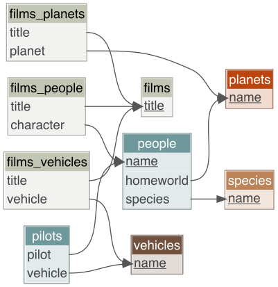

Select all films with characters whose homeworld is Kamino.
Filter the people table to only contain humans from Tatooine and export the result to a CSV file called “folks.csv”.
Close the SQL connection.

SQL

David Gerard

2023-11-06

Learning Objectives

SQL Introduction and Motivation

DuckDB

Basic SQL

General

Showing Tables

Select Specific Columns

Filter rows

Arranging Rows

Mutate

Group Summaries

Creating Grouped Summaries without Grouping the Results

Recoding

Joining

Creating some Tables

Tidyr stuff

Writing Tables to a CSV File

Passing SQL output to R in R Markdown

Calling SQL from R

Use R to generate SQL with `{dbplyr}`

Closing the Connection

Exercises

SQL

David Gerard

2023-11-06

Learning Objectives

SQL Introduction and Motivation

DuckDB

Basic SQL

General

Showing Tables

Select Specific Columns

Filter rows

Arranging Rows

Mutate

Group Summaries

Creating Grouped Summaries without Grouping the Results

Recoding

Joining

Creating some Tables

Tidyr stuff

Writing Tables to a CSV File

Passing SQL output to R in R Markdown

Calling SQL from R

Use R to generate SQL with {dbplyr}

Closing the Connection

Exercises

Use R to generate SQL with `{dbplyr}`