Data Manipulation with Pandas

Author

David Gerard

Published

June 3, 2025

Learning Objectives

Read in and manipulate data with pandas.
Chapter 3 of Python Data Science Handbook.

Python Overview

In R I Want	In Python I Use
Base R	numpy
dplyr/tidyr	pandas
ggplot2	matplotlib/seaborn

Pandas versus Tidyverse

These are the equivalencies you should have in mind.

<DataFrame>.fun() means that fun() is a method of the <DataFrame> object.

<Series>.fun() means that fun() is a method of the <Series> object.

tidyverse	pandas
`arrange()`	`<DataFrame>.sort_values()`
`bind_rows()`	`pandas.concat()`
`filter()`	`<DataFrame>.query()`
`gather()` and `pivot_longer()`	`<DataFrame>.melt()`
`glimpse()`	`<DataFrame>.info()` and `<DataFrame>.head()`
`group_by()`	`<DataFrame>.groupby()`
`if_else()`	`numpy.where()`
`left_join()`	`pandas.merge()`
`library()`	`import`
`mutate()`	`<DataFrame>.eval()` and `<DataFrame>.assign()`
`read_csv()`	`pandas.read_csv()`
`recode()`	`<DataFrame>.replace()`
`rename()`	`<DataFrame>.rename()`
`select()`	`<DataFrame>.filter()` and `<DataFrame>.drop()`
`separate()`	`<Series>.str.split()`
`slice()`	`<DataFrame>.iloc()`
`spread()` and `pivot_wider()`	`<DataFrame>.pivot_table().reset_index()`
`summarize()`	`<DataFrame>.agg()`
`unite()`	`<Series>.str.cat()`
`\|>`	Enclose pipeline in `()`

Importing libraries

Python: import <package> as <alias>.

Python
```
import numpy as np
import pandas as pd
```
You can use the alias that you define in place of the package name. In Python we write down the package name a lot, so it is nice for it to be short.
R equivalent

R
```
library(tidyverse)
```

Reading in and Printing Data

We’ll demonstrate most methods with the “estate” data that we’ve seen before: https://data-science-master.github.io/lectures/data/estate.csv
You can read about these data here: https://data-science-master.github.io/lectures/data.html
Python: pd.read_csv(). There is a family of reading functions in pandas (fixed width files, e.g.). Use tab-completion to scroll through them.

Python
```
estate = pd.read_csv("../data/estate.csv")
```

R equivalent:

estate <- read_csv("../data/estate.csv")

Use the info() and head() methods to get a view of the data.

Python

estate.info()

<class 'pandas.core.frame.DataFrame'>
RangeIndex: 522 entries, 0 to 521
Data columns (total 12 columns):
 #   Column   Non-Null Count  Dtype 
---  ------   --------------  ----- 
 0   Price    522 non-null    int64 
 1   Area     522 non-null    int64 
 2   Bed      522 non-null    int64 
 3   Bath     522 non-null    int64 
 4   AC       522 non-null    int64 
 5   Garage   522 non-null    int64 
 6   Pool     522 non-null    int64 
 7   Year     522 non-null    int64 
 8   Quality  522 non-null    object
 9   Style    522 non-null    int64 
 10  Lot      522 non-null    int64 
 11  Highway  522 non-null    int64 
dtypes: int64(11), object(1)
memory usage: 49.1+ KB

Python

estate.head()

    Price  Area  Bed  Bath  AC  ...  Year  Quality  Style    Lot  Highway
0  360000  3032    4     4   1  ...  1972   Medium      1  22221        0
1  340000  2058    4     2   1  ...  1976   Medium      1  22912        0
2  250000  1780    4     3   1  ...  1980   Medium      1  21345        0
3  205500  1638    4     2   1  ...  1963   Medium      1  17342        0
4  275500  2196    4     3   1  ...  1968   Medium      7  21786        0

[5 rows x 12 columns]

R equivalent:

glimpse(estate)

Rows: 522
Columns: 12
$ Price   <dbl> 360000, 340000, 250000, 205500, 275500, 248000, 229900, 150000…
$ Area    <dbl> 3032, 2058, 1780, 1638, 2196, 1966, 2216, 1597, 1622, 1976, 28…
$ Bed     <dbl> 4, 4, 4, 4, 4, 4, 3, 2, 3, 3, 7, 3, 5, 5, 3, 5, 2, 3, 4, 3, 4,…
$ Bath    <dbl> 4, 2, 3, 2, 3, 3, 2, 1, 2, 3, 5, 4, 4, 4, 3, 5, 2, 4, 3, 3, 3,…
$ AC      <dbl> 1, 1, 1, 1, 1, 1, 1, 1, 1, 0, 0, 1, 1, 1, 1, 1, 1, 1, 1, 1, 1,…
$ Garage  <dbl> 2, 2, 2, 2, 2, 5, 2, 1, 2, 1, 2, 3, 3, 2, 2, 2, 2, 2, 2, 2, 2,…
$ Pool    <dbl> 0, 0, 0, 0, 0, 1, 0, 0, 0, 0, 1, 0, 0, 0, 0, 0, 0, 0, 0, 0, 0,…
$ Year    <dbl> 1972, 1976, 1980, 1963, 1968, 1972, 1972, 1955, 1975, 1918, 19…
$ Quality <chr> "Medium", "Medium", "Medium", "Medium", "Medium", "Medium", "M…
$ Style   <dbl> 1, 1, 1, 1, 7, 1, 7, 1, 1, 1, 7, 1, 7, 5, 1, 6, 1, 7, 7, 1, 2,…
$ Lot     <dbl> 22221, 22912, 21345, 17342, 21786, 18902, 18639, 22112, 14321,…
$ Highway <dbl> 0, 0, 0, 0, 0, 0, 0, 0, 0, 0, 0, 0, 0, 0, 0, 0, 0, 0, 0, 0, 0,…

`DataFrames` and `Series`

Pandas reads in tabular data as a DataFrame object.
Just as R’s data.frame is a list of a bunch of vectors, Panda’s DataFrame contains a bunch of Series objects.
A Series object is a generalization of a numpy array. So you can use numpy functions on it.

Python
```
x = pd.Series([1, 4, 2, 1])
x[2:3]
x[pd.Series([0, 2])]
x[x >= 2]
np.sum(x)
```

Extract Variables

Python: Use a period. This extracts the column as a Pandas Series.

Python
```
estate.Price
```
Then you can use all of those numpy functions on the Series

Python
```
np.mean(estate.Price)
np.max(estate.Price)
```
R equivalent: Use a $:

R
```
estate$Price
```

Filtering/Arranging Rows (Observations)

Filter rows based on booleans (logicals) with query(). The queries need to be in quotes.

Python
```
estate.query('(Price > 300000) & (Area < 2500)')
```
Some folks use bracket notation, which is more similar to base R

Python
```
estate[(estate.Price > 300000) & (estate.Area < 2500)]
```

R equivalent:

filter(estate, Price > 300000, Area < 2500)

Select rows by numerical indices with iloc()

Python

estate.iloc[[1, 4, 10]]

     Price  Area  Bed  Bath  AC  ...  Year  Quality  Style    Lot  Highway
1   340000  2058    4     2   1  ...  1976   Medium      1  22912        0
4   275500  2196    4     3   1  ...  1968   Medium      7  21786        0
10  190000  2812    7     5   0  ...  1966      Low      7  56639        0

[3 rows x 12 columns]

R equivalent:

slice(estate, 1, 4, 10)

# A tibble: 3 × 12
   Price  Area   Bed  Bath    AC Garage  Pool  Year Quality Style   Lot Highway
   <dbl> <dbl> <dbl> <dbl> <dbl>  <dbl> <dbl> <dbl> <chr>   <dbl> <dbl>   <dbl>
1 360000  3032     4     4     1      2     0  1972 Medium      1 22221       0
2 205500  1638     4     2     1      2     0  1963 Medium      1 17342       0
3 160000  1976     3     3     0      1     0  1918 Low         1 32358       0

Arrange rows by sort_values().

Python

estate.sort_values(by="Price", ascending=False)

R equivalent

R
```
arrange(estate, desc(Price))
```
Exercise: Use both the tidyverse and pandas to extract all medium quality homes that have a pool and arrange the rows in increasing order of price.

Selecting Columns (Variables)

Variables are selected using filter().

Python

estate.filter(["Price"])
estate.filter(["Price", "Area"])

Some folks use bracket notation, which is more similar to Base R.

Python
```
estate[["Price"]]
estate[["Price", "Area"]]
```
The inner brackets [] just creates a Python list. The outer brackets [] says that we are subsetting the columns.

R equivalent:

select(estate, Price)
select(estate, Price, Area)

Dropping a column is done by drop(). The axis=1 argument says to drop by columns (rather than by “index”, which is something we haven’t covered).

Python
```
estate.drop(["Price", "Area"], axis=1)
```
R: just use select() with a minus sign.

R
```
select(estate, -Price, -Area)
```

Renaming variables is done with rename().

Python

estate.rename({'Price': 'price', 'Area': 'area'}, axis = 'columns')

R equivalence:

rename(estate, price = Price, area = Area)

# A tibble: 522 × 12
    price  area   Bed  Bath    AC Garage  Pool  Year Quality Style   Lot Highway
    <dbl> <dbl> <dbl> <dbl> <dbl>  <dbl> <dbl> <dbl> <chr>   <dbl> <dbl>   <dbl>
 1 360000  3032     4     4     1      2     0  1972 Medium      1 22221       0
 2 340000  2058     4     2     1      2     0  1976 Medium      1 22912       0
 3 250000  1780     4     3     1      2     0  1980 Medium      1 21345       0
 4 205500  1638     4     2     1      2     0  1963 Medium      1 17342       0
 5 275500  2196     4     3     1      2     0  1968 Medium      7 21786       0
 6 248000  1966     4     3     1      5     1  1972 Medium      1 18902       0
 7 229900  2216     3     2     1      2     0  1972 Medium      7 18639       0
 8 150000  1597     2     1     1      1     0  1955 Medium      1 22112       0
 9 195000  1622     3     2     1      2     0  1975 Low         1 14321       0
10 160000  1976     3     3     0      1     0  1918 Low         1 32358       0
# ℹ 512 more rows

Exercise: Use the tidyverse and pandas to select year, price, and area.

Creating New Variables (Mutate)

New variables are created in Python using eval(). Note that we need to place the expression in quotes.

Python
```
estate.eval('age = 2013 - Year')
```
You can use assign(), but then you need to reference the DataFrame as you extract variables:

Python
```
estate.assign(age = 2013 - estate.Year)
```
R equivalent:

R
```
mutate(estate, age = 2013 - Year)
```
Exercise: Use the tidyverse and pandas to calculate the price per unit area.

Piping

All of these pandas functions return DataFrames. So, we can apply methods to these DataFrames by just appending methods to the end.
- This is called “method chaining”.
E.g., suppose we want to find the total number of beds/baths and only select the price and this total number to print. Then the following code would work.

Python
```
estate.eval('tot = Bed + Bath').filter(["Price", "tot"])
```
If you want to place these operations on different lines, then just place the whole operation within parentheses.

Python
```
(
estate.eval('tot = Bed + Bath')
  .filter(["Price", "tot"])
)
```

This looks similar to piping in the tidyverse

estate |>
  mutate(tot = Bed + Bath) |>
  select(Price, tot)

Exercise: Use pandas to extract all medium quality homes that have a pool and arrange the rows in increasing order of price. Use piping.

Group Summaries

Summaries can be calculated by the agg() method. You usually first select the columns whose summaries you want before running agg().

Python

(
estate.filter(["Price", "Area"])
  .agg(np.mean)
)

<string>:3: FutureWarning: The provided callable <function mean at 0x1210c3130> is currently using DataFrame.mean. In a future version of pandas, the provided callable will be used directly. To keep current behavior pass the string "mean" instead.
Price    277894.147510
Area       2260.626437
dtype: float64

R equivalent

summarize(estate, Price = mean(Price), Area = mean(Area))

# A tibble: 1 × 2
    Price  Area
    <dbl> <dbl>
1 277894. 2261.

Use groupby() to create group summaries.

Python

(
estate.filter(["Price", "Area", "Bed", "Bath"])
  .groupby(["Bed", "Bath"])
  .agg(np.mean)
)

R equivalent

estate |>
  group_by(Bed, Bath) |>
  summarize(Price = mean(Price), Area = mean(Area))

You can get multiple summaries out by passing a list of functions:

Python

(
estate.filter(["Price", "Area", "Quality"])
  .groupby("Quality")
  .agg([np.mean, np.var])
)

You can create your own functions and pass those

Python

def cv(x):
  """Calculate coefficient of variation"""
  return(np.sqrt(np.var(x)) / np.mean(x))

(
estate.filter(["Price", "Area"])
  .agg(cv)
)

Price    0.495841
Area     0.314242
dtype: float64

Recoding

Use replace() with a dict object to recode variable values.

Python
```
estate.replace({'AC' : {0: "No AC", 1: "AC"}})
```

R equivalent:

estate |>
  mutate(AC = recode(AC,
                     "0" = "No AC",
                     "1" = "AC"))

To recode values based on logical conditions, use np.where().

Python

estate.assign(isbig = np.where(estate.Price > 300000, "expensive", "cheap"))

R equivalence:

mutate(estate, isbig = if_else(Price > 300000, "expensive", "cheap"))

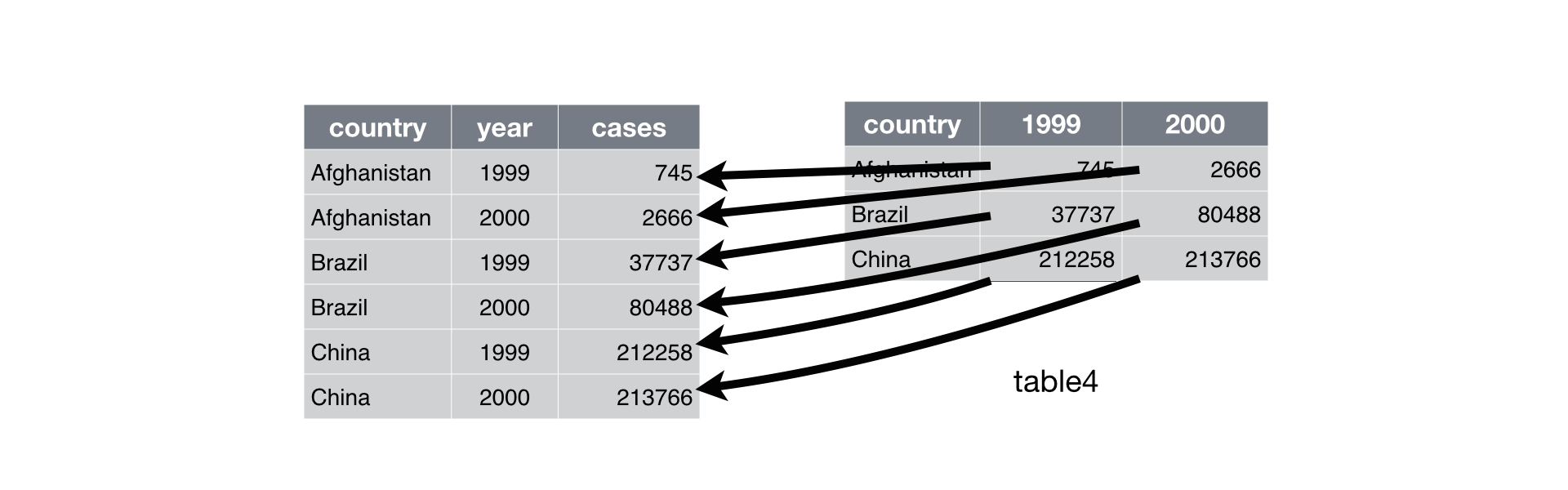
Gathering

Problem: One variable spread across multiple columns.
Column names are actually values of a variable

Recall table4a from the tidyr package

data("table4a")

Python

table4a = pd.DataFrame({'country': ['Afghanistan', 'Brazil', 'China'],
                        '1999': [745, 37737, 212258],
                        '2000': [2666, 80488, 213766]})
table4a

       country    1999    2000
0  Afghanistan     745    2666
1       Brazil   37737   80488
2        China  212258  213766

Solution: melt().

Python

table4a.melt(id_vars='country', value_vars=['1999', '2000'])

       country variable   value
0  Afghanistan     1999     745
1       Brazil     1999   37737
2        China     1999  212258
3  Afghanistan     2000    2666
4       Brazil     2000   80488
5        China     2000  213766

R equivalences:

gather(table4a, key = "variable", value = "value", `1999`, `2000`)

# A tibble: 6 × 3
  country     variable  value
  <chr>       <chr>     <dbl>
1 Afghanistan 1999        745
2 Brazil      1999      37737
3 China       1999     212258
4 Afghanistan 2000       2666
5 Brazil      2000      80488
6 China       2000     213766

pivot_longer(table4a, cols = c("1999", "2000"), 
             names_to = "variable",
             values_to = "value")

# A tibble: 6 × 3
  country     variable  value
  <chr>       <chr>     <dbl>
1 Afghanistan 1999        745
2 Afghanistan 2000       2666
3 Brazil      1999      37737
4 Brazil      2000      80488
5 China       1999     212258
6 China       2000     213766

RDS visualization:
Exercise: Use pandas to gather the monkeymem data frame (available at https://data-science-master.github.io/lectures/data/tidy_exercise/monkeymem.csv). The cell values represent identification accuracy of some objects (in percent of 20 trials).

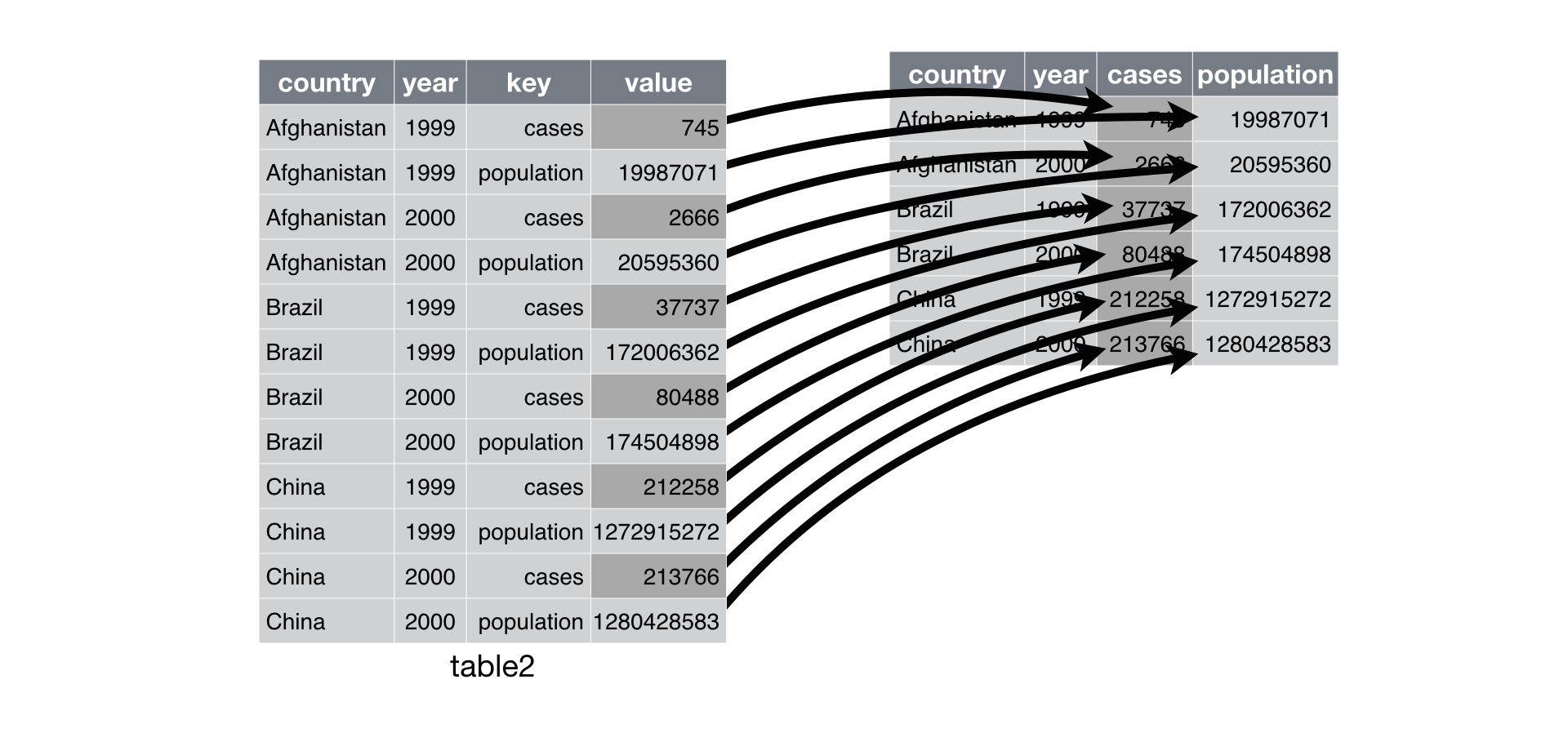
Spreading

Problem: One observation is spread across multiple rows.
One column contains variable names. One column contains values for the different variables.

Recall table2 from the tidyr package

data("table2")

Python

table2 = pd.DataFrame({'country': ['Afghanistan', 'Afghanistan', 
                                   'Afghanistan', 'Afghanistan', 
                                   'Brazil', 'Brazil', 'Brazil', 
                                   'Brazil', 'China', 'China', 
                                   'China', 'China'],
                       'year': [1999, 1999, 2000, 2000, 1999, 1999, 
                                2000, 2000, 1999, 1999, 2000, 2000],
                       'type': ['cases', 'population', 'cases', 
                                'population', 'cases', 'population', 
                                'cases', 'population', 'cases', 
                                'population', 'cases', 'population'],
                       'count': [745, 19987071, 2666, 20595360, 37737,
                                 172006362, 80488, 174504898, 212258, 
                                 1272915272, 213766, 1280428583]})
table2

        country  year        type       count
0   Afghanistan  1999       cases         745
1   Afghanistan  1999  population    19987071
2   Afghanistan  2000       cases        2666
3   Afghanistan  2000  population    20595360
4        Brazil  1999       cases       37737
5        Brazil  1999  population   172006362
6        Brazil  2000       cases       80488
7        Brazil  2000  population   174504898
8         China  1999       cases      212258
9         China  1999  population  1272915272
10        China  2000       cases      213766
11        China  2000  population  1280428583

Solution: pivot_table() followed by reset_index().

Python

(
table2.pivot_table(index=['country', 'year'], columns='type', values='count')
  .reset_index()
)

type      country  year     cases    population
0     Afghanistan  1999     745.0  1.998707e+07
1     Afghanistan  2000    2666.0  2.059536e+07
2          Brazil  1999   37737.0  1.720064e+08
3          Brazil  2000   80488.0  1.745049e+08
4           China  1999  212258.0  1.272915e+09
5           China  2000  213766.0  1.280429e+09

pivot_table() creates a table with an index attribute defined by the columns you pass to the index argument. The reset_index() converts that attribute to columns and changes the index attribute to a sequence [0, 1, ..., n-1].

R equivalences

spread(table2, key = "type", value = "count")

# A tibble: 6 × 4
  country      year  cases population
  <chr>       <dbl>  <dbl>      <dbl>
1 Afghanistan  1999    745   19987071
2 Afghanistan  2000   2666   20595360
3 Brazil       1999  37737  172006362
4 Brazil       2000  80488  174504898
5 China        1999 212258 1272915272
6 China        2000 213766 1280428583

pivot_wider(table2, id_cols = c("country", "year"), 
            names_from = "type", 
            values_from = "count")

# A tibble: 6 × 4
  country      year  cases population
  <chr>       <dbl>  <dbl>      <dbl>
1 Afghanistan  1999    745   19987071
2 Afghanistan  2000   2666   20595360
3 Brazil       1999  37737  172006362
4 Brazil       2000  80488  174504898
5 China        1999 212258 1272915272
6 China        2000 213766 1280428583

RDS visualization:
Exercise: Use pandas to spread the flowers1 data frame (available at https://data-science-master.github.io/lectures/data/tidy_exercise/flowers1.csv).

Separating

Sometimes we want to split a column based on a delimiter:

data("table3")

Python

table3 = pd.DataFrame({'country': ['Afghanistan', 'Afghanistan', 'Brazil', 
                                   'Brazil', 'China', 'China'],
                       'year': [1999, 2000, 1999, 2000, 1999, 2000],
                       'rate': ['745/19987071', '2666/20595360', 
                                '37737/172006362', '80488/174504898', 
                                '212258/1272915272', '213766/1280428583']})
table3

       country  year               rate
0  Afghanistan  1999       745/19987071
1  Afghanistan  2000      2666/20595360
2       Brazil  1999    37737/172006362
3       Brazil  2000    80488/174504898
4        China  1999  212258/1272915272
5        China  2000  213766/1280428583

Python

table3[['cases', 'population']] = table3.rate.str.split(pat = '/', expand = True)
table3.drop('rate', axis=1)

       country  year   cases  population
0  Afghanistan  1999     745    19987071
1  Afghanistan  2000    2666    20595360
2       Brazil  1999   37737   172006362
3       Brazil  2000   80488   174504898
4        China  1999  212258  1272915272
5        China  2000  213766  1280428583

R equivalence

separate(table3, col = "rate", sep = "/", into = c("cases", "population"))

# A tibble: 6 × 4
  country      year cases  population
  <chr>       <dbl> <chr>  <chr>     
1 Afghanistan  1999 745    19987071  
2 Afghanistan  2000 2666   20595360  
3 Brazil       1999 37737  172006362 
4 Brazil       2000 80488  174504898 
5 China        1999 212258 1272915272
6 China        2000 213766 1280428583

Exercise: Use pandas to separate the flowers2 data frame (available at https://data-science-master.github.io/lectures/data/tidy_exercise/flowers2.csv).

Uniting

Sometimes we want to combine two columns of strings into one column.

data("table5")

Python

table5 = pd.DataFrame({'country': ['Afghanistan', 'Afghanistan', 'Brazil',
                                   'Brazil', 'China', 'China'], 
                       'century': ['19', '20', '19', '20', '19', '20'], 
                       'year': ['99', '00', '99', '00', '99', '00'], 
                       'rate': ['745/19987071', '2666/20595360', 
                                '37737/172006362', '80488/174504898', 
                                '212258/1272915272', '213766/1280428583']})
table5

       country century year               rate
0  Afghanistan      19   99       745/19987071
1  Afghanistan      20   00      2666/20595360
2       Brazil      19   99    37737/172006362
3       Brazil      20   00    80488/174504898
4        China      19   99  212258/1272915272
5        China      20   00  213766/1280428583

You can use str.cat() to combine two columns.

Python

(
table5.assign(year = table5.century.str.cat(table5.year))
  .drop('century', axis = 1)
)

       country  year               rate
0  Afghanistan  1999       745/19987071
1  Afghanistan  2000      2666/20595360
2       Brazil  1999    37737/172006362
3       Brazil  2000    80488/174504898
4        China  1999  212258/1272915272
5        China  2000  213766/1280428583

R equivalence:

unite(table5, century, year, col = "year", sep = "")

# A tibble: 6 × 3
  country     year  rate             
  <chr>       <chr> <chr>            
1 Afghanistan 1999  745/19987071     
2 Afghanistan 2000  2666/20595360    
3 Brazil      1999  37737/172006362  
4 Brazil      2000  80488/174504898  
5 China       1999  212258/1272915272
6 China       2000  213766/1280428583

Exercise: Use pandas to re-unite the data frame you separated from the flowers2 exercise. Use a comma for the separator.

Joining

We will use these DataFrames for the examples below.

Python

xdf = pd.DataFrame({"mykey": np.array([1, 2, 3]), 
                    "x": np.array(["x1", "x2", "x3"])})
ydf = pd.DataFrame({"mykey": np.array([1, 2, 4]), 
                    "y": np.array(["y1", "y2", "y3"])})
xdf
ydf

xdf <- tibble(mykey = c("1", "2", "3"),
              x_val = c("x1", "x2", "x3"))
ydf <- tibble(mykey = c("1", "2", "4"),
              y_val = c("y1", "y2", "y3"))
xdf
ydf

Binding rows is done with pd.concat().

Python
```
pd.concat([xdf, ydf])
```
R equivalence:

R
```
bind_rows(xdf, ydf)
```
All joins use pd.merge().

Inner Join (visualization from RDS):

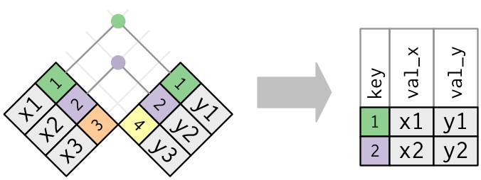
Python

pd.merge(left=xdf, right=ydf, how="inner", on="mykey")

inner_join(xdf, ydf, by = "mykey")

Outer Joins (visualization from RDS):

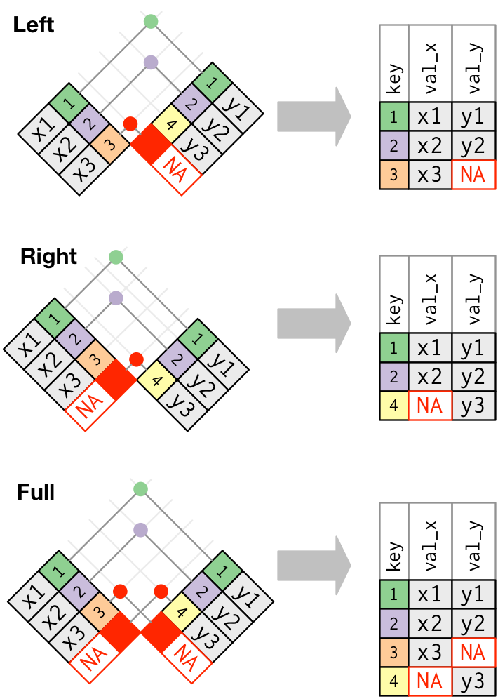
Left Join

Python

pd.merge(left=xdf, right=ydf, how="left", on="mykey")

left_join(xdf, ydf, by = "mykey")

Right Join

Python

pd.merge(left=xdf, right=ydf, how="right", on="mykey")

right_join(xdf, ydf, by = "mykey")

Full Join

Python

pd.merge(left=xdf, right=ydf, how="outer", on="mykey")

full_join(xdf, ydf, by = "mykey")

Use the left_on and right_on arguments if the keys are named differently.
The on argument can take a list of key names if your key is multiple columns.

Extra Resources

I am not an expert in Python, and there is so much more to Python than what I am presenting here. Here are some resources if you want to learn more:
Python Data Science Handbook
Python for Data Analysis
Another Book on Data Science

Learning Objectives

Python Overview

Pandas versus Tidyverse

Importing libraries

Reading in and Printing Data

DataFrames and Series

Extract Variables

Filtering/Arranging Rows (Observations)

Selecting Columns (Variables)

Creating New Variables (Mutate)

Piping

Group Summaries

Recoding

Gathering

Spreading

Separating

Uniting

Joining

Extra Resources

`DataFrames` and `Series`